Introduction

Building upon our previous exploration of Logistic Regression by using the Maximum Likelihood , this article will guide you through the practical implementation of these concepts. Understanding how to translate mathematical equations into working code is a crucial skill for anyone interested in machine learning and deep learning.

We'll implement gradient descent for logistic regression using PyTorch, one of the most popular deep learning frameworks. Along the way, we'll address common challenges that arise when moving from theory to practice, with particular focus on addressing numerical stability issues that can impact model performance.

Generating synthetic data for learning

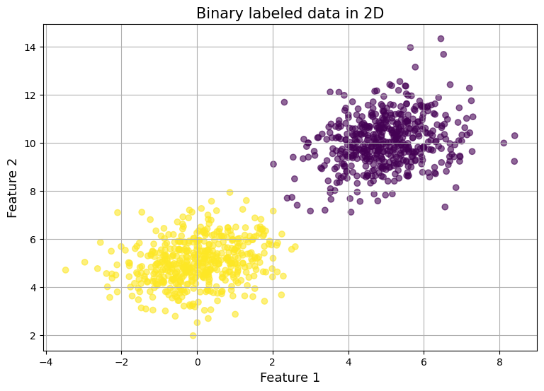
To validate our model's effectiveness and facilitate debugging, we'll first generate synthetic training data. We'll create a two-dimensional dataset using multivariate normal distributions, with two distinct classes for our binary classification task.

We only require three imports:

import torch
import matplotlib.pyplot as plt
import numpy as np
torch.manual_seed(0); # Ensure reproducibility

PyTorch requires all data to be in tensor format with explicit data types. We'll generate 500 samples for each class, with the data points distributed in 2D space using a covariance of 0.25:

n_samples = torch.tensor(500)
covariance = torch.tensor([[1, 0.25],  [0.25, 1]])

To create distinguishable classes, we'll separate them by setting different mean values for each:

mean_class_one = torch.tensor([5,10],dtype=torch.float32)
mean_class_two = torch.tensor([0, 5],dtype=torch.float32)

With PyTorch's MultivariateNormal distribution function, we can randomly generate feature points:

dist_class_one = torch.distributions.MultivariateNormal(loc=mean_class_one, covariance_matrix=covariance)
class_one_features = dist_class_one.rsample(sample_shape=(n_samples,))
dist_class_two = torch.distributions.MultivariateNormal(loc=mean_class_two, covariance_matrix=covariance)
class_two_features = dist_class_two.rsample(sample_shape=(n_samples,))

Finally, we'll combine our features and create corresponding labels.

Note: The random seed we set earlier ensures reproducibility of these results:

features = torch.vstack((class_one_features, class_two_features))
labels = torch.hstack((-torch.ones(n_samples), torch.ones(n_samples))).reshape((-1,1))
print(f'features shape: {features.shape}')
print(f'labes shape {labels.shape}')
'''
features shape: torch.Size([1000, 2]) 
labes shape torch.Size([1000, 1])
'''

Sigmoid Function Implementation

While PyTorch provides a built-in sigmoid function, implementing our own version helps us understand important numerical considerations. Let's start with the basic implementation:

def sigmoid(z):
    return 1 / (1+torch.exp(-z))

When we test this implementation with both small and large values, PyTorch appears to handle the computation smoothly:

arr_sm = torch.randn(size=(1,10))
arr_lg = arr_sm*-1000
print(sigmoid(arr_sm)) # tensor([[...]])
print(sigmoid(arr_lg)) # tensor([[...]])

However, PyTorch's smooth handling masks an important numerical stability issue. To understand this better, let's compare with NumPy's behavior:

def sigmoid_np(z):
    return 1/(1+np.exp(-z))

print(sigmoid_np(arr_lg))
'''
RuntimeWarning: overflow encountered in exp
  return 1/(1+np.exp(-z))
array([[...]])
'''

The NumPy implementation reveals a critical numerical stability issue through its runtime warning. This occurs due to limitations in floating-point arithmetic:

When calculating exp(1000), we encounter an overflow problem. The result is too large to be represented in standard floating-point format.
Conversely, exp(-1000) produces a very small number close to zero, which can be represented accurately in memory.

Understanding these numerical stability issues is crucial when implementing machine learning algorithms, as they can significantly impact model training and performance. In our next section, we'll explore how to implement a numerically stable version of the sigmoid function.

Fixing Numerical Instability for the Sigmoid Function

The overflow of sigmoid(x) stems from handling large negative numbers. The issue arises because we are calculating $e^{-x}$ , which behaves differently across the number line:

As $x$ decreases, $e^{-x}$ approaches infinity and as $x$ increases, $e^{-x}$ approaches $0$ .

\begin{align} \lim_{x -> -\infty} e^{-x} = \infty \\ \lim_{x -> \infty} e^{-x} = 0 \\ \end{align}

This behavior suggests we should only use the formula $1/(1+e^{-x})$ when $x \geq 0$ .

For large negative values of $x$ , we need an alternative formulation that avoids calculating $e^{-(-x)}$ .

Deriving this alternative form leverages a fundamental property of the sigmoid function:

\begin{align} \sigma(-x) = 1 - \sigma(x) \end{align}

With some algebraic manipulation, we can derive the alternative form:

\begin{align*} \sigma(-x) &=& 1 - \sigma(x) \\ \sigma(x) &=& 1 - \sigma(-x) \\ \sigma(x) &=& 1 - \frac{1}{1+e^x} \\ \sigma(x) &=& \frac{e^x}{1+e^x} \\ \end{align*}

Note that this form of the sigmoid function should only be used when $x<0$ to prevent overflow issues with large positive numbers. Here is the numpy implementation:

def sigmoid_stable_np(z):
    mask = z >= 0
    result = np.zeros_like(z)
    result[mask] = 1 / (1 + np.exp(-z[mask]))
    result[~mask] = np.exp(z[~mask]) / (1 + np.exp(z[~mask]))
    return result

sigmoid_stable_np(arr_lg.numpy())
'''
array([[...]])
'''

Note: No RuntimeWarning this time.

Since PyTorch doesn't provide overflow warnings by default, we'll create a helper function to detect these issues:

def warn_exp(z):
    ans = torch.exp(z)
    if torch.any(torch.isinf(ans)):
        print("Overflow detected: result is infinity.")
    return ans
print(warn_exp(arr_lg))
'''
Overflow detected: result is infinity. 
tensor([[...]])
'''

Finally, here's our numerically stable implementation in PyTorch:

def sigmoid_stable(z):
    mask = z >= 0
    result = torch.zeros_like(z)
    result[mask] = 1 / (1 + warn_exp(-z[mask]))
    result[~mask] = warn_exp(z[~mask]) / (1 + warn_exp(z[~mask]))
    return result
print(sigmoid_stable(arr_lg))
''' 
tensor([[...]])
'''

No overflow warning confirms that our implementation of PyTorch handles the numerical stability issues with large exponents.

Exercise: Compare our implementation to the PyTorch implementation of the sigmoid function (torch.nn.Sigmoid). Consider testing these implementations with normal range values, extreme negative values, and extreme positive values.

Questions to Consider:

Do all implementations produce the same results for normal-range inputs?
How do the implementations handle extreme values?
Are there any differences in numerical precision between the implementations?
What advantages might PyTorch's implementation offer?

What is the effect of the Sigmoid Function on our Feature Space?

To understand how the sigmoid function transforms our data, let's visualize its effect on our feature space. This visualization will provide crucial insights into how our model processes the input data.

fs = sigmoid_stable(features)
plt.figure(figsize=(9, 6))
plt.scatter(fs[:, 0], fs[:, 1],
            c=labels, alpha=.6);

plt.title("Binary labeled data in 2D", size=15);
plt.xlabel("Feature 1", size=13);
plt.ylabel("Feature 2", size=13);
plt.grid();

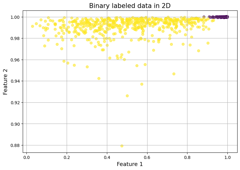The sigmoid function compresses all values into the range $[0,1]$ on both axes, creating a bounded feature space. Second, the transformation has created an interesting asymmetry in our class distribution. The points labeled as -1 are concentrated in the upper-right region of the plot, appearing more densely clustered. In contrast, the points labeled as 1 exhibit a more dispersed distribution across the transformed space.

Logistic Regression Forward Pass

In this section, we'll walk through the forward pass of a logistic regression model step by step. Our model has two parameters: $w$ (weights) and $b$ (bias). To begin, we initialize both to zero:

w = torch.zeros((features.shape[1], 1))
b = torch.zeros(1)
print(f'{w.flatten()=}, {b=}')
# w.flatten()=tensor([0., 0.]), b=tensor([0.])

Note: In deep learning, initializing all parameters to zero is not a good practice because it can lead to getting stuck in local minima when optimizing non-convex functions. Instead, weights are typically initialized randomly.

With our model parameters we can compute the predictions:

def y_pred(X, w, b=0):
    result = sigmoid_stable(X @ w + b)
    return result

Understanding the Forward Pass

The forward pass outputs a probability for each data point, indicating its confidence in the likelihood of the label being $1$ . Let us see our initial predictions:

predictions = y_pred(features, w=w, b=b)
print(predictions[:5])
'''
tensor([[0.5000],
        [0.5000],
        [0.5000],
        [0.5000],
        [0.5000]])
'''

The model is unsure about what the actual label is since the probability is $0.5$ for all samples.

Converting Probabilities to Labels

To test the accuracy of our model we need to convert the probability values into binary label values. We will assume the following:

if $p \geq 0.5$ then the class is $1$
Otherwise, classify the label as $-1$ .

predicted_labels = torch.where(predictions >= 0.5, 1, -1)
print(predicted_labels[:5])
'''
tensor([[1],
        [1],
        [1],
        [1],
        [1]])
'''

Right now the model thinks all data points are label $1$ giving us an accuracy of $0.5$ .

accuracy = (predicted_labels == labels).sum() / labels.shape[0]
print(f'Accuracy {accuracy:.4f} (want close to 1)')
# Accuracy 0.5000 (want close to 1)

We can also look at the log loss:

print(f'Negative Log Loss Sum: {-predictions.log().sum():.4f} (want close to 0)')
print(f'Negative Log Loss Average: {-predictions.log().mean():.4f} (want close to 0)')
'''
Negative Log Loss Sum: 693.1473 (want close to 0)
Negative Log Loss Average: 0.6931 (want close to 0)
'''

Since we will be looking at these metrics frequently, lets create a helper function for this:

def accuracy(predictions, labels):
    predicted_labels = torch.where(predictions > 0.5, 1, -1)
    return (predicted_labels == labels).sum() / labels.shape[0]

def lls(predictions):
    return -predictions.log().sum()

Handling Numerical Instability

Consider the log loss of the following predictions:

arr_unstable = torch.tensor([1.0, 0.9, 0.0])

An issue arises when we take the $\log(0)$ . This is because $\lim_{x->0^+} \log(x) = -\infty$ . This instability is related to the sigmoid instability because $\log(x)$ is an inverse to $e^x$ .

To prevent this instability, we will clamp values within a small range $\epsilon$ to avoid extreme probabilities. We will also create another helper function to detect if an overflow occured.

def warn_log(z):
    ans = torch.log(z)
    if torch.any(torch.isinf(ans)):
        print("Overflow detected: result is infinity.")
    return ans

ep = 10e-10
def lls(predictions):
    return -warn_log(torch.clamp(predictions, ep, 1-ep)).sum()

Sanity Check: Should not get a warning.

lls(unstable_array)
# tensor(103.6163)

The function below will also help us visualize our model predicitons:

def analyze_model_preds(features, labels, w,b):
    predictions = y_pred(features, w=w, b=b)
    predicted_labels = torch.where(predictions > 0.5, 1, -1)
    plt.figure(figsize=(9, 6))
    plt.scatter(features[:, 0], features[:, 1],
                c=predicted_labels, alpha=.6);

    plt.title("Binary labeled data in 2D", size=15);
    plt.xlabel("Feature 1", size=13);
    plt.ylabel("Feature 2", size=13);
    plt.grid();

    acc = accuracy(predictions, labels)
    print(f'Accuracy {acc:.4f} (want close to 1)')
    log_loss_sum = lls(predictions)
    print(f'Negative Log Loss Sum: {log_loss_sum:.4f} (want close to 0)')
    print(f'Negative Log Loss Average: {log_loss_sum/len(predictions):.4f} (want close to 0)')

Calculate the Gradients and Update Model Parameters

Calculate Gradients

The gradient values for the weights and bias are calculated from the functions below:

\begin{align} \frac{\partial NLL}{\partial \mathbf{w}} = - \sum_{i=1}^n \sigma \left( - y_i \left( \mathbf{w}^\top \mathbf{x}_i + b \right) \right) \cdot y_i \mathbf{x}_i \\ \frac{d NLL(\mathbf{X},\mathbf{y},\mathbf{w}, b)}{db}=- \sum_{i=1}^n y_i \sigma \left(-y_i \left( \mathbf{w}^\top\mathbf{x}_i + b \right) \right) \end{align}

Let us initialize and compute the forward pass:

w = torch.zeros((features.shape[1],1))
b = torch.tensor(0.0)
linear_pred = (features@w+b)
activation = sigmoid_stable(-labels*linear_pred)

With the forward pass, we can calculate the gradients of $w$ and $b$ :

wgrad = -1*torch.sum(activation*labels*features,dim=0, keepdim=True).T
bgrad = -1*torch.sum(activation*labels)
print(f'{wgrad=}, {bgrad=}')
'''
wgrad=tensor([[1245.4592],
        [1253.0986]]), bgrad=tensor(-0.)
'''

Common Pitfall: Ensure that you sum across the correct dimension when computing weight gradients.

Exercise: What is the difference between dim=0 vs. dim=1 when calculating the gradients for $w$ ?

To get better intuition on tensor dimension watch Andrej Karpathy's makemore Tutorials

Update Model parameters

Notice that $w$ has large gradient values while $b$ remains small. To prevent drastic updates, we use a learning rate:

learning_rate = 0.01
print(f'Before: {w.flatten()=} {b=}')
w -= learning_rate*wgrad
b -= learning_rate*bgrad 
print(f'After: {w.flatten()=} {b=}')
''' 
Before: w.flatten()=tensor([0., 0.]) b=tensor(0.) After: w.flatten()=tensor([-12.4546, -12.5310]) b=tensor(0.)
'''

We update our model parameters opposite the direction of the gradient to minimize loss.

Gradient Function

def gradient(X, y, w, b):
    _, d = X.shape
    wgrad = torch.zeros((d, 1))
    bgrad = torch.tensor(0.0)

    linear_preds = X@w+b
    activation = sigmoid_stable(-y*linear_preds)

    # weights gradients 
    d_dw = activation * y*X
    wgrad = -1*torch.sum(d_dw, dim=0, keepdim=True).T

    # bias gradient
    bgrad = -1*torch.sum(activation*y)
    
    return wgrad, bgrad

Training the Logistic Regression Model

max_iter = 10
w = torch.zeros((features.shape[1] ,1))
b = torch.tensor(0.0)
loss_over_iter = []
accurary_over_iter = []
learning_rate = torch.tensor(0.1)
ep = 1e-10

for step in range(max_iter):

    wgrad, bgrad = gradient(features, labels, w, b)

    w -= learning_rate * wgrad
    b -= learning_rate* bgrad
    linear_preds = features @ w + b
    activation = sigmoid_stable(linear_preds * labels)

    nll = lls(activation).item()
    avg_nll = nll/labels.shape[0]
    loss_over_iter.append(avg_nll)
    acc = accuracy(y_pred(features, w, b), labels).item()
    accurary_over_iter.append(acc)
    print(f'Accuracy={acc:.4f} Total NLL={nll:.4f} Average NLL={avg_nll:.4f}')
'''
Accuracy=0.5000 Total NLL=11512.9258 Average NLL=11.5129
Accuracy=0.5000 Total NLL=11512.9248 Average NLL=11.5129
Accuracy=0.5000 Total NLL=11512.9258 Average NLL=11.5129
Accuracy=0.5400 Total NLL=10565.9541 Average NLL=10.5660
Accuracy=0.9630 Total NLL=807.4803 Average NLL=0.8075
Accuracy=0.9710 Total NLL=640.7943 Average NLL=0.6408
Accuracy=0.9680 Total NLL=683.8399 Average NLL=0.6838
Accuracy=0.9680 Total NLL=615.8058 Average NLL=0.6158
Accuracy=0.9720 Total NLL=641.5195 Average NLL=0.6415
Accuracy=0.9670 Total NLL=631.1148 Average NLL=0.6311
'''

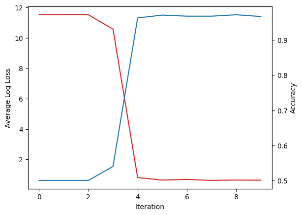
After $10$ iterations, we observe a drastic improvement in our metrics. Accuracy went from $0.5$ to $0.96$ and loss went from $11$ to $0.6$ . Lets plot the change:

fig, ax1 = plt.subplots()
ax1.plot(loss_over_iter, color="tab:red")
ax1.set_xlabel('Iteration')
ax1.set_ylabel('Average Log Loss')

ax2 = ax1.twinx() 
ax2.plot(accurary_over_iter, color="tab:blue")
ax2.set_ylabel('Accuracy')

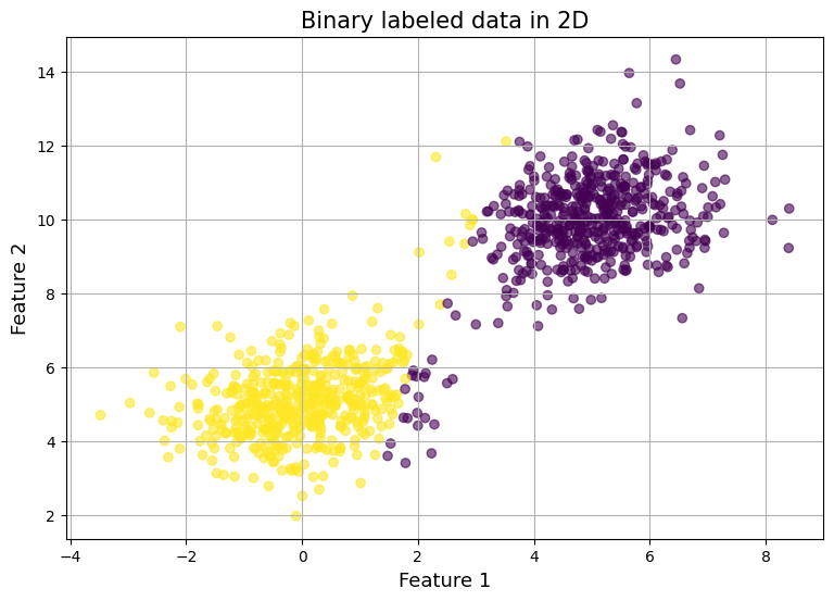
Graph of our feature space shows that the model is having some difficulty classifying labels with high variance.

Logistic Regression Training Function

from tqdm import tqdm 

def logistic_regression(features, labels, max_iter=100, learning_rate=1e-1):
    w = torch.zeros((features.shape[1] ,1))
    b = torch.tensor(0.0)
    loss_over_iter = []
    accurary_over_iter = []

    for _ in tqdm(range(max_iter)):

        wgrad, bgrad = gradient(features, labels, w, b)

        w -= learning_rate * wgrad
        b -= learning_rate* bgrad
        linear_preds = features @ w + b
        activation = sigmoid_stable(linear_preds * labels)

        nll = lls(activation).item()
        avg_nll = nll/labels.shape[0]
        loss_over_iter.append(avg_nll)
        acc = accuracy(y_pred(features, w, b), labels).item()
        accurary_over_iter.append(acc)
    return w, b, [loss_over_iter, accurary_over_iter]

Lets train over $1,000$ iterations:

w, b, [loss_history, acc_history] = logistic_regression(features, labels, max_iter=10, learning_rate=0.01)
analyze_model_preds(features, labels, w, b)

Output:

Accuracy 0.9690 (want close to 1) Negative Log Loss Sum: 11220.8330 (want close to 0) Negative Log Loss Average: 11.2208 (want close to 0)

Graph:

Conclusion

In this post, we explored the forward and backward passes of logistic regression, derived gradients, and implemented gradient descent to train our model. Through this process, we translated theory into practice, iteratively deepening our understanding of logistic regression.

Additionally, we refactored our code to make our experiments reproducible. By adjusting parameters, we observed improvements in accuracy and reductions in loss. Visualizing the results confirmed that our model was learning effectively.

Check out this github repo for the code written in this blog.

Farooq A. Khan